Gabor Vali - May 24, 2002
[A virtual colloquium -- I just wish I could use a pointer! ]
The main reason for interest in this case, and prompting this posting of analyses, is that very little drizzle was present in the cloud, and therefore the WCR data can be used to explore vertical motions with negligible contributions from particle fall velocities.
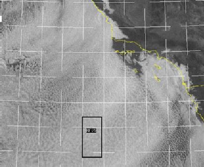
Satellite images show the cloud field to be quite uniform in the study area. Fine cellular structure is clearly evident in the early morning visible image (below). A band of speckle in the NRL lowloud images traverses the study area all night. An image loop is avaliable through this link.
Soundings show an inversion of about 10°C, low mixing ratios in a shallow layer above and higher and more variable humidity by about 1200 m altitude:
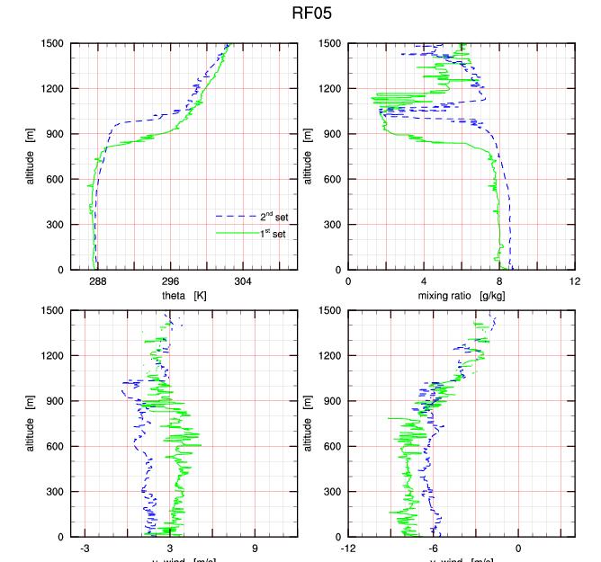
It may be of interest to note that during the 10:30 - 10:58 UTC circle above the cloud, at 998 m altitude and about 100 m above cloud top, there was a large difference in humidity between the south-eastern and north-western parts of the circle, with interesting transitions between the regions. This was accompanied by about a 1K change in THETA. These temperature and humidity variations are shown in the two lowermost panels of Fig. 1. The same figure shows intersting correlations between echo top height, the radiative surface temperature (RSTB) and the upwelling IR flux (IRBC).
Cloud top from the SABL measurements was: 828 ± 42 m during the 07:36 - 08:06 circle, 816 ± 36 m during the 10:30 - 10:58 circle, and 959 ± 35 m during the 13:54 - 14:19 circle. These numbers indicate a significant change during the latter part of the flight and there is more evidence for that from the in situ data to be discussed later. During the first and last circles, cloud top altitude showed large-scale variations with azimuth. This was not the case during the 10:30 - 10:58 circle when variance in cloud top altitude was dominated by relatively small horizontal scales.
Cloud thickness, from aircraft soundings and from the radar images, varied around 250 m. The LWC maxima were near 0.5 g m-3. The FSSP wasn't working, but the Fast-FSSP was. Total drop concentrations are in the 100 to 160 cm-3 range. The data from the 1D and 2D probes look quite clean, without problems due to artifacts. These data indicate maximum drizzle drop sizes increasing with time from about 150 um during the first two in-cloud circles around 09:00, to near 350 um diameter during the final in-cloud circle started at 12:30, all the while in very low concentrations. Just after the 10:30 - 10:58 "radar" circle, the maximum drizzle size (from visual scrutiny of the 2D records) was 200 um, with a total number of about 10 during the whole half-hour track. With these spectral characteristics and with the observed radar reflectivity, the reflectivity-weighted fall velocity is about 2 cm s-1. It is the small magnitude of this fall velocity that justifies the assertion made in the introductory paragraph.
Radar reflectivity imagesare shown in Fig. 2. (a pdf file with 4 pages). As the image shows, an upward gradient is clearly evident nearly everywhere. That is expected for a case where the reflectivity is dominated by increasing liquid water content and cloud droplets of increasing sizes toward the cloud top. There are also some breaks in the cloud. The lidar data confirms that these are complete breaks; lidar edge detection indicated only the ocean surface at these points. Echo coverage, based on the radar data, was 90-95%, from the lidar data it was close to 98%; the difference is due to the sensitivity limitaion of the radar.
The mean reflectivity profile, and the corresponding precipitation rate (from Z-R conversion) are shown in Fig. 3.
For proper appreciation of these data, it should be remembered that the radar data has a vertical resolution of 15 m (from doubly oversampling the 30-m rangegate spacing) and has been here averaged to 9.5 m horizontal spacing between profiles. In the middle of the cloud, the sample volume for one pixel of radar data is, nominally, 570 m3. Data are displayed here for values exceeding -30 dBZ, the minimum detectable signal for the cloud layer given a noise threshold of -21.8 dBZ at 1 km.
As in other cases, the vertical mean reflectivity, VMZ, is correlated with echo top height. This is shown in Fig. 4 with the upper panel showing points for 10-m segments in the horizontal, and the lower panel for 1-km horizontal averages. The correlation is stronger (r = 0.84) for 1-km averages due to variations on larger scales. Fig. 1 shows these large-scale variations (upper two panels in figure), depicted in terms of azimuth along the flight circle. Measurements of upwelling radiation are also included (middle panels); these too indicate the presence of small breaks in the cloud.
Vertical velocity are shown in Fig. 5 in an analogous format to the reflectivities shown in Fig. 2. The two figures have identical scales and can be displayed side by side for comparison. Velocity data are accepted only for points where the reflectivity exceeds -30 dBZ. Vertical velocities shown here are those of hydrometeors, so that they are a combination of air velocity and drop fall velocity (reflectivity weighted, i.e. dominated by the larger drops to a degree depending on the shape of the size spectrum). Aircraft motion and the component of horizontal winds along the nadir beam have been removed from these velocities.
The radar-measured velocities, Vr, display considerably more variation in the horizontal than is seen in the reflectivities. Maxima and minima in velocities are also surprisingly high: the absolute extremes are +4.3 and -4.0 m s-1 (positive is upward). The 0.1, 1, 99 and 99.9 percentiles are -2.71, -1.73, +1.76 and 2.78 m s-1. Remembering the large sample size involved (over 300,000 pixels in cloud) and the large sample volume per pixel, these values are significant. For the in-cloud circles just following the data segment shown here, the standard deviation of the aircraft-measured vertical air velocities is 0.68 m s-1. That value compares well with the 0.66 m s-1 from the radar velocities, further reinforcing the point that the contribution of droplet fall velocities has a negligible effect in this case. The extreme velocities indicated by the 25 Hz aircraft data are roughly of the magnitude of the 0.1 and 99.9 percentile values from the radar. The smaller sample volume of the aircraft measurement explains why the radar-measured values extend the tails of the distributions beyond the values indicated by the in situ data, by more than 1 m s-1 in either direction. However, the larger coverage of the cloud volume by the radar could have been expected to be offset by the larger averaging of turbulent velocities involved in the radar measurement, so these results indicate that those very rare but large velocities are occurring on scales of tens of meters.
The frequency distribution of Vr is shown in Fig. 6, in two different forms. The larger diagram shows the fraction of cloud volume that has velocity values exceeding in magnitude the values given by the ordinate. The inset figure shows how close the cumulative form of the distribution is to a Gaussian shown with dashed lines. The striking thing about the distribution is the smooth and uniform extension of frequencies toward the tails. Since this is the first such analysis of the radar data, it is an open question to what degree this finding can be generalized.
The differential form of the distribution is shown in Fig. 7. Here, the upper panel shows the frequency per bin of 0.2 m s-1 width. The lower panel shows the first moment of the distribution, i.e. the relative contribution that different velocities make to the vertical flux of air. The flux values are on an arbitrary scale, for lack of a good basis to assign a horizontal dimension over which the measured Vr can be assumed to be valid (a minimum estimate for this number is provided by the horizontal cross-section of the radar beam, which averages 38 m2 at mid-cloud, from a rectangle of 4 x 9.5 m.) In any event, the shape of this distribution reveals that the dominant velocities from the flux perspective are near ±0.5 m s-1.
All these comments about Vr raise the question just how precise these measurements are. In lieu of a simple answer, which is not in hand yet, perhaps the best indication is the noise we observe for the vertical velocity of the ocean surface. The typical value of the standard deviation of surface velocities is around 0.25 m s-1 and the range of maxima to minima is about 1 m s-1. Since these values include an unknown contribution by actual velocities of wave motion, they represent an upper limit for the noisiness of Vr. Thus, a few tenth of m s-1 may be taken as a rough statement of precision. Most of the imprecision derives from incomplete removal of aircraft motion, plus there is the inherent phase noise of the radar hardware. More work is needed to characterize these terms.
In addition to the individual point values of Vr, I have looked at the vertical mean velocity VMVEL, i.e. the average of Vr along vertical lines through the cloud. In spite of the fact that the velocities are by no means uniform along these vertical lines, the shape of the frequency distribution of VMVEL values is indistinguishable from a Gaussian. The standard deviation of the distribution is 0.47 m s-1; this value is much larger than the value that random sampling of groups of 15 points (the average number of rangegates in cloud along a vertical) would have.
Interesting deductions can be made from looking at the correlation between VMZ (vertical mean of reflectivity) and VMVEL. This is shown in Figs. 8a. and 8b.. The same data are represented in these two figures and the upper panels are identical. The lower panel in Fig 8a shows the mean value of VMVEL and its 10 and 90 percentiles for 2-dBZ intervals of VMZ. In reverse, the lower panel in Fig 8b shows mean values ofVMZ and its 10 and 90 percentiles for intervals of 0.4 m s-1 inVMVEL. The numbers by each set of points indicate the corresponding sample sizes. The two diagrams make the same point in slightly different ways: higher reflectivities correspond to larger velocities. Lower values of VMZ coincide with negative values of VMVEL. The trend is accentuated, though not entirely caused by two regions of points distinguishable in the otherwise overcrowded scatterplots of the upper panels. First, there is a group of points in the zone roughly bounded by -23 to -20 dBZ and 0.7 to 2.0 m s-1. These points indicate cloud regions with high average vertical velocities and strong reflectivities, suggesting that these regions have liquid water contents closest to adiabatic, and, perhaps, lower cloud bases than other regions. Second, there is a set of points with low reflectivities and negative velocities; these points are directly interpretable as indicating reduced LWC associated with entrainment and evaporation. These linkages are not surprising; documentation of the effects reinforce and quantify them, but leave open the questions of cause and effect.
There is another correlation of interest, and can be readily seen even by inspection of the velocity images in Fig. 5: cloud tops are higher where vertical velocities are strong. This pattern is quantified in Fig. 9, using the same display form as in Fig. 8. While it is natural to expect higher cloud tops for larger vertical velocities, the nearly 50 m range, from 850 to 900 m, where the effect is most pronounced, is probably much larger than could be accounted for by additional kinetic energy moving the cloud upward. Here again, there is clear ambiguity between cause and effect, because vertical velocities in the cloud are likely to be reinforced by gravity waves or other phenomena above the inversion.
A first look at the horizontal scales of variabilities in VMVEL is given in Fig. 10 showing the frequencies of contiguous patches in which the indicated limits are exceeded. The limits are the 10, 20, 30, 40, 60, 70, 80 and 90 percentiles of VMVEL. For all the threshold values, small patch sizes dominate, and there is no hint of any preferred scale of these mean velocities.
The locations and shapes of more intense updrafts and downdrafts clearly deserve special attention. While the statistics presented earlier are good measures of the overall picture, it is useful to see specific manifestations of the events. As one step in that direction, images are given in Fig. 11 which have cloud regions with velocities exceeding 1 m s-1 and those inferior to -1 m s-1 highlighted with a special color scheme. In this figure, two image strips are to be read simultaneously, moving from the upper pair to the lower pair and then onto the next page. Perhaps the most readily evident feature revealed by this figure -- also there in Fig. 5 but harder to see -- is that the majority of updraft and downdraft regions are located in the lower part of the cloud. Some updraft regions reach to the upper 2/3 of the cloud, and some are quite massive, like those seen at 10:41:25, 10:44:28 or 10:54:23. Examples of narrow and deep updrafts can be seen at 10:33:30, 10:35:55, 10:43:17, and others. Somewhat surprisingly, the stronger downdrafts shown in this figure do not occur on either side of already existing breaks in the cloud. Downdrafts even more than updrafts are located near the lower boundary of the cloud. (A caveat is in order: cloud of low LWC may extend below the -30 dBZ zones depicted in these figures.) Striking exceptions, with highlighted zones extending from cloud top all the way to the bottom, and corresponding to depressions in cloud top height, are seen at 10:35:40, 10:38:20 and 10:51:52. An almost general pattern is that the highlighted downdraft regions correspond to downward bulges in the bottom boundary of the echo (cloud).
This is how far the analyses have gone, for now. More to follow. But, thanks are not to be delayed: to S. Haimov, D. Leon, the NCAR/RAF and all of DYCOMS.
_______________________________________________
Click here to go to Part 2 of this
report.