Solar radiation, albedo and climate

B. Geerts

1/'02

A case of alternative regimes of climate can be described in terms of a change of surface albedo.

The albedo controls the amount of heat absorbed by the Earth, available for heating the surface air through infrared radiation and sensible heat flux. For simplicity, assume that the Earth has no oceans and no clouds. If the Earth surface is green foliage, with an albedo around 0.22, 78% of the incoming shortwave radiation is available to heat the air, apart from what is used in evaporation and longwave radiation into space, which are assumed constant for this exercise. However, only about 20% is available if the surface is ice, because of its much higher albedo.

Now examine the increase of incoming solar radiation (Q_s) as one moves from an ice-covered polar region towards lower latitudes. As long as there is ice, the temperature rises only slowly with increasing Q_s, about a quarter as much as when the surface is green. Two lines representing these alternatives are shown in Fig 1; the slopes have a ratio of 78:20 (about 4:1).

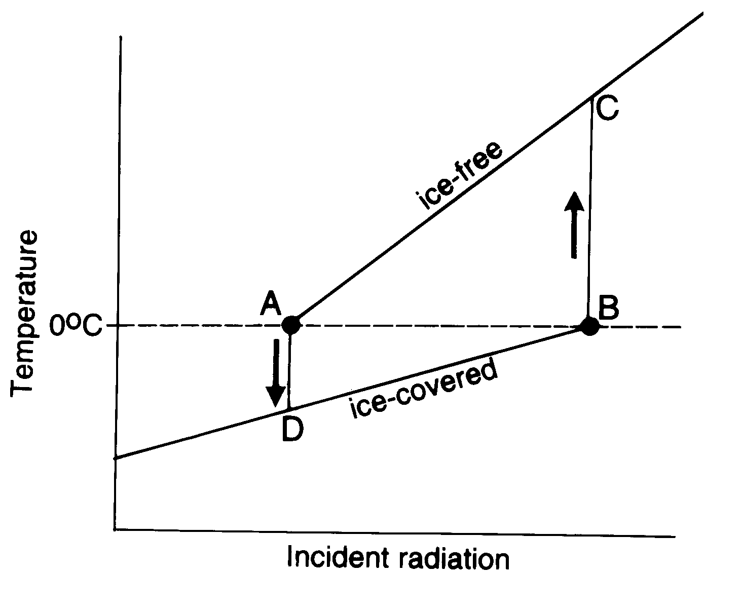
Fig 1. Diagram of the effect of the amount of solar radiation on the surface temperature, according to the surface albedo.

What is most interesting about Fig 1 is the relationship of the two lines to the freezing point, and what happens when a change of cloudiness or solar constant, for instance, alters Q_s. In the case of an ice covered surface, an enhanced Q_s causes warming until the situation is represented by B, at which point the ice melts, and the temperature suddenly increases to C. If then there is a decrease of Q_s, the temperature falls towards A in the diagram. If the cooling is sufficient and A is reached, there is a sudden cooling to D.

It may be seen that C and D represent fairly stable situations, with no change of surface until some large excursion of Q_s causes a change to either A or B, respectively. Then there is a sudden flip to the alternative regime. This is an example of a system which is ‘almost intransitive’, i.e. it alternates irregularly between prolonged periods in one or other of two different states (1). The Pleistocene has witnessed a flip-flopping between glacials and interglacials, with large ice sheets building and disappearing at latitudes were the mean temperature is near freezing.

The diagram also indicates that the rise is likely to be more dramatic than the onset of ice, i.e. an Ice Age ends more quickly than it begins. At the end of the Younger Dryas about 11 kBP the Arctic warmed by about 7 K in only 50 years (2). There the change of albedo would be from 80% of ice to 6% of the ocean, i.e. even greater than from ice to foliage.

The slope of the line for the foliage case in Fig 1 corresponds to conditions where the latitude (f, in degrees) is lower than about 60 degrees, where the following equation obtains -

Tc / Q_s = 0.146 - 0.0017 f

K.m²/watt

where Tc is the sea-level annual mean temperature (3).

It may be noted that Tc is related empirically to latitude approximately as follows (4) -

Tc = 27 - 0.008 f² ºC

This indicates that the sea-level annual-mean temperature is 0ºC at about 58 degrees latitude. The almost intransitive climate is most applicable to conditions around this latitude. Nearer the pole, there is ice more often than not and the reduced available solar radiation leads to lower temperatures (i.e. between D and B in Fig 1).

References

(1) Linacre, E.T. 1969. Empirical relationships involving the global radiation intensity and ambient temperature at various latitudes and altitudes. Archiv. Meteor. Geophys. Bioklimatol. B 17, 1-20.

(2) Linacre, E.T. 1992. Climate Data & Resources (Routledge) 366pp.

(3) McGuffie, K. & A. Henderson-Sellers 1997. A Climate Modelling Primer (John Wiley & Sons) 253pp.

(4) Houghton, J. 1994. Global Warming: the complete briefing (Lion Publishing plc, Oxford) 192pp.